
- Date: January 25, 2020
- Categories: PCB Layout and Design
Short Summary
|
1. INTRODUCTION 1.1 Task 1.2 Project Objective 2. How to Detect Small Capacitive Changes? 2.1 Servo Amplifier 2.2 Conclusion on Voltage Dependency on Capacitance 2.3 Precision AC to DC Converter 2.4 Conclusion on Capacitance for Different Dielectric Constants 2.5 Conclusion on Amplification Dependency on Dielectric Constant 2.6 Conclusion on Capacitance Dependency on Water Level and Dielectric Constant 3. Implementation 3.1 Further Possible Implementations 4. Alternative Linearization Method 5. Possible Sensor Applications 6. Electrical Connection Scheme 7. Literature 7.1 Simulation and Design Programs |
1. INTRODUCTION
This report serves as a finals project for subject “Measurement of Non-electrical Quantities”, within the framework of developing a product specialized for industrial development and use. This project is described from the research phase to the final prototype, including all the problems that had to be solved in order to construct the final product.
1.1 Task
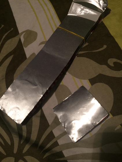
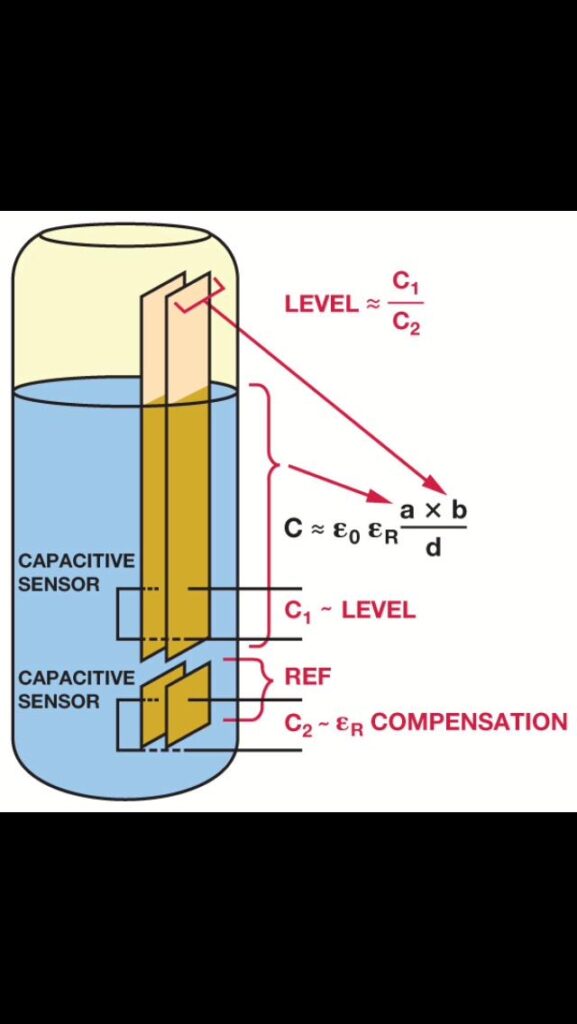
For the subject “Measurement of Non-electrical Quantities”, we constructed a custom sensor for measuring levels (Figure 1a). After constructing the physical sensor and confirming that it gives a change in physical quantity at its output, it is necessary to create a measuring transducer that will convert the non-standard quantity into a standard measuring quantity.
1.2 Project Objective
Our project goal was to demonstrate the knowledge we gained during our four years of study at the faculty and to show that we understood everything we learned during our studies in the professional field.
2. How to Detect Small Capacitive Changes?
This is a complex issue because our capacitance sensor has a capacitance in the order of pico (10p-12p) Farads. Such values are very difficult to measure, especially to detect with conventional measuring instruments. We started solving this problem using a 555 timer, but through calculation, we realized that we where going to be pushing the frequency limits of this timer. The biggest problem was the small capacitance, which theoretically had a maximum value of about 10pF (for the best case), and for the minimum value, we couldn’t even notice those changes. According to the frequency calculation formula, it would exceed 600 kHz, which is beyond the range defined by the manufacturer. However, based on the graph (Figure 6), it can be concluded that the dielectric constant has a significant influence on the sensor’s capacitance. We wanted to avoid the measurement result depending on the dielectric constant of the liquid, so we designed a compensator. Here, another problem arose because there is no function with which we can multiply the output frequency to avoid dependence on the dielectric constant. After consulting with our mentor, we concluded that this was not the best solution and that it could not give us consistent results, and the final result would depend on the dielectric constant. When i went back to the drawing boards, i thought carefully about what could have enough sensitivity to detect such small changes. We concluded that the most precise way would be to measure the capacitance change with a servo amplifier, where at the output, we obtain two alternating voltages that need to be passed through a “precision AC to DC converter”.
2.1 Servo Amplifier
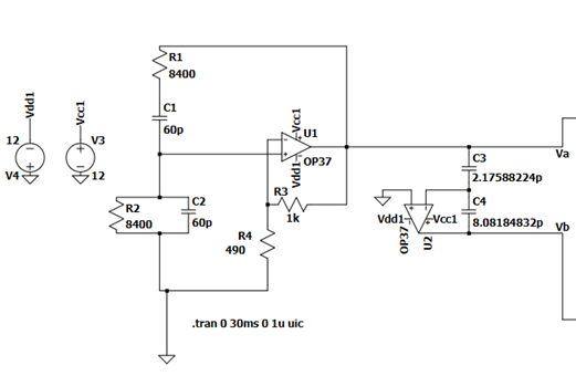
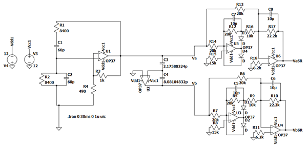
After further research, i concluded that we need a voltage ratio that will depend on the ratio of two capacitances. We achieved this using a servo amplifier where the sensor is in negative feedback, and the compensator with a power supply is connected to the feedback loop (Figure 2). The next configuration gives us the desired output voltage.
2.2 Conclusion on Voltage Dependency on Capacitance
Depending on the capacitance, there will be a change in voltage at the output of the servo amplifier. This voltage can be seen from the simulation in Figures 3a) and 3b).
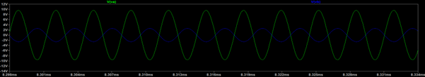
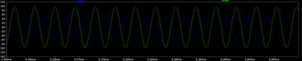
We conclude that the voltage will increase (dark blue alternating line) as the level decreases. AC-DC conversion is required to measure this voltage.
2.3 Precision AC to DC Converter
To convert alternating voltage to direct current, we use a precision voltage rectifier circuit (Figure 4). This circuit differs from standard rectifier circuits in that they can rectify very small voltage values, whereas standard rectifiers are limited by diode voltages, which can cause problems when rectifying smaller voltages.
2.4 Conclusion on Capacitance for Different Dielectric Constants
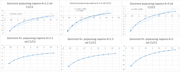
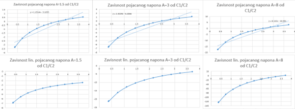
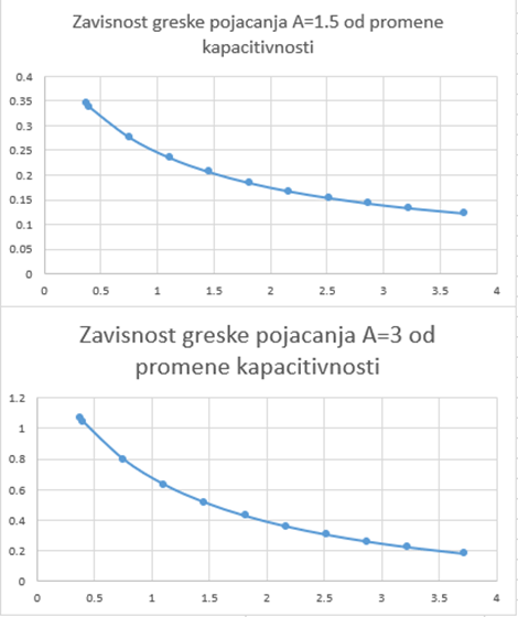
After experimenting for a while, we concluded that our capacitance increases with the increase in dielectric constant. Designing circuits becomes more complex as the dielectric constant decreases. For hydrazine, which has the smallest dielectric constant we worked with (ε = 52), the higher the gain (A), the more linear the dependence of capacitance on the voltage difference in the measuring bridge. For water with a medium dielectric constant (ε = 78.4), we noticed that the higher the gain, the less linear it is; we tried gains of A = 1.5 and A = 15, and this can be seen from the graphs (Figure 5). From the graphs and voltage, it can be concluded that the best gain is in the range from A = 1.2 to A = 1.5. The acceptable error is 5%, and the voltage is in the standard range of 0 V – 10 V. For formamide, which has the highest constant we worked with (ε = 109), the situation is the same as for water; the higher the gain, the more nonlinear the dependence of capacitance on voltage (Figure 6). For specific numbers and more detailed graphs, refer to the Excel tables for the dielectric constant of interest.
2.5 Conclusion on Gain Dependency on Dielectric Constant
For small dielectric constants, capacitance is small, so the voltage gain must be higher, and the curve becomes more non-linear, increasing the error. For higher dielectric constants in the range of ε = 75 to ε = 110, we need less gain, making it easier for practical application in experiments, thus reducing the error. The higher the gain needed, the greater the error. This can be observed in Figure 6. The higher the gain, the greater the error; the amplifier amplifies everything, including the error.
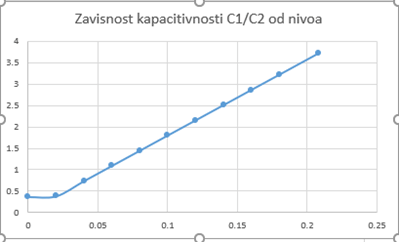
2.6 Conclusion on Capacitance Dependency on Water Level and Dielectric Constant
In addition to the height, capacitance will also depend on the dielectric constant according to the formula (Figure 7a).
3. Implementation
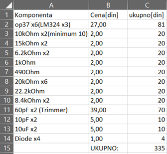
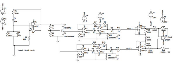
After completing the design of the electrical scheme (Figure 8), we created a table of all the components we use, the BOM table (Figure 9). We obtained the components from Orbit electronics and Sprint electronics in Novi Sad.
The connection and calibration of the device were carried out in a laboratory located in the building of the “Naučno tehnološki park” in Novi Sad. Figure 10a) and 10b) show the testing of the alternating voltage generator at 300 kHz and its average value.
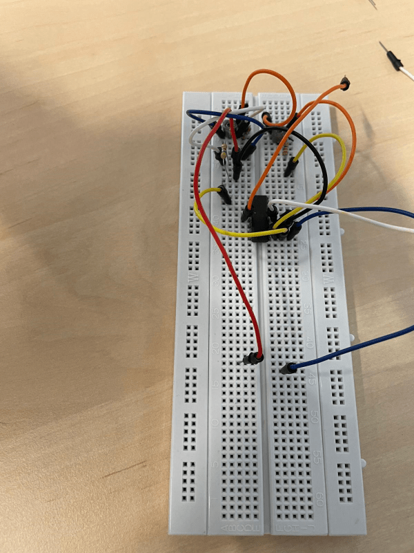
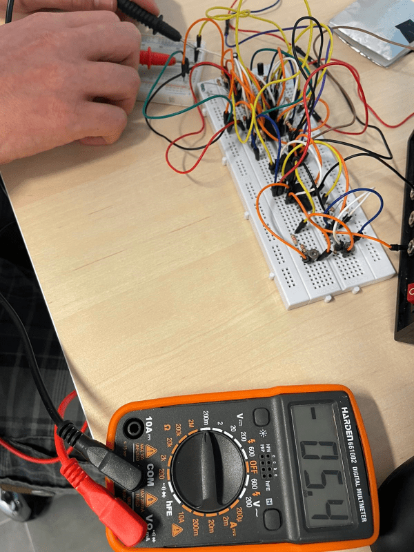
After confirming that the sinusoidal generator works, we proceeded with further testing. The next step is to test the output of the servo amplifier (Figure 11a and 11b). The connection of the level sensor and the compensator was done using short-circuit connectors, and constant contact was maintained using insulating tape. We then followed the electrical scheme and made the necessary connections. The final result can be seen in Figures 11a) and 11b).
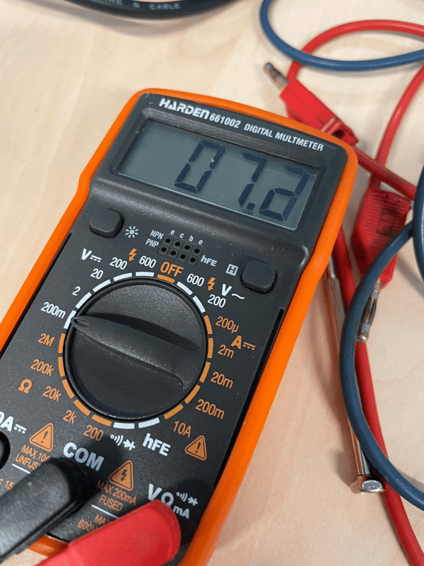
After verifying that the servo amplifier works and gives an output voltage, it is necessary to rectify the voltage coming out of the servo amplifier. For this purpose, we use a precision AC-DC rectifier (Figure 12a).

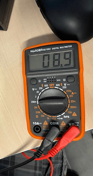
After verifying that the rectifier works, we connected it to the rectifier for the servo amplifier. First, the measurement of the minimum level was performed, the sensor and compensator were dry, and the measurement result is shown in Figure 12b)
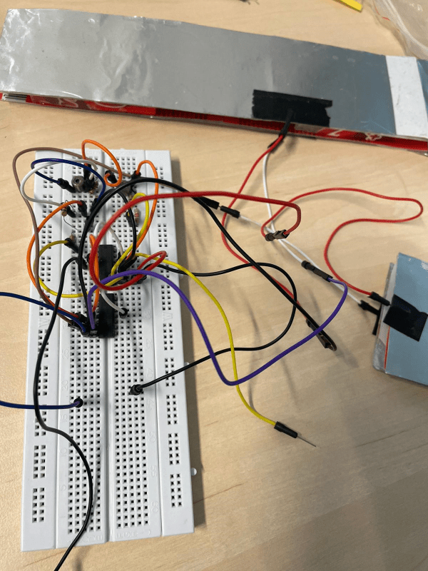
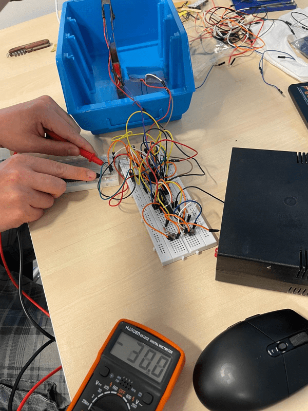
The next step is to immerse the sensor and check the output voltage. The voltage increased when we submerged our sensor; the output voltage can be seen in Figure 12c)
3.1 Further Possible Implementation
This project can be further implemented by dividing the voltage of the sinusoidal generator and the output voltage of the servo amplifier. This is possible with logarithmic amplifiers, but their complexity is too high for this course.
4. Alternative Linearization
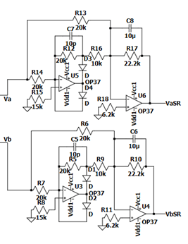
There is another possibility for linearizing this sensor, instead of a servo amplifier and logarithmic amplifier, a measuring bridge is added to the electrical scheme, and an instrumentation amplifier is added that will use the voltage from the resistor branch as a reference (the voltage is constant), and the ratio of two capacitances will create a voltage difference in the bridge, further calculation determines the components of the instrumentation amplifier so that its output ranges from 0 V to 10 V. Figure 13 represents the electrical scheme of how this method could look.
5. Possible Sensor Applications
Measuring of:
Formamide: Dielectric constant: 109 Temperature [K]: 293; Temperature [°C]: 19.85 Gain: A=1.5
Sulfuric Acid: Dielectric Constant: 84 to 100 (85 for our case) Temperature [K]: 293.15 to 278.15; Temperature [°C]: 20 to 25 Gain: A=1.5
Water: Dielectric Constant: 78.4 Temperature [K]: 298; Temperature [°C]: 24.85 Gain: A=1.5
Hydrazine: Dielectric Constant: 52.0 Temperature [K]: 293.15; Temperature [°C]: 20 Gain: A=1.5
Source of dielectric constants for given temperatures Wikipedia
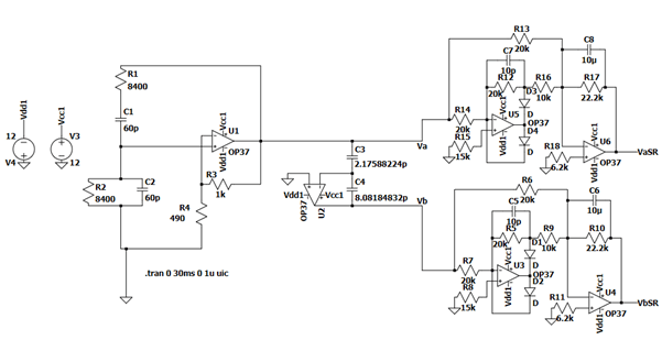
6. Electrical Connection Scheme
Final electrical connection scheme (Figure 14) for connecting the level sensor prototype linearization.
7. Literature
[1] A DESIGNER’S GUIDE TOINSTRUMENTATION AMPLIFIERS by Charles Kitchin and Lew Counts 3RD Edition [2] Nonlinear circuit handbook bz The Engineering Staff of Analog Devices, Inc. Edited by Daniel H. Shingold [3] An IC Amplifier User’s Guide to Decoupling, Grounding,and Making Things Go Right for a Change By Paul Brokaw [4] Designing Operational Amplifier Oscillator Circuits For Sensor Applications by Jim Lepkowski
7.1 Simulation and Design Programs
[1] LTSpice [2] Proteus 8 professional